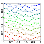
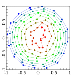
This is a test level as well as the previous one. It is a relatively large map so the portal culling comes quite in handy in this case.
I went down the rabbit hole too deep trying to improve sampling in my light mapper running on ray tracing hardware. Found some random generators suitable for GPU usage, and also adapted a sampling method on the way.
This material is a byproduct of a ray tracing research project I was working on quite a while ago. The project goal was to write a light mapper using IMG’s ray tracing hardware. We wanted to publish our results in a short paper, but it just did not survived the review process unfortunately. Since hardware accelerated ray tracing has became a hype lately big time, I thought it would worth it to share some of the ideas I had during and after the project.
It started with a textbook implementation of a path tracer to compute diffuse radiance, using some typical cosine weighted, low-discrepancy random sampling to shoot rays around from each light map texel. The hardware did its job nicely, but obviously, the process was far from optimal. After some performance analysis, it became clear that the biggest issue was the system memory bandwidth caused by the large number of incoherent rays. Even if the hardware is designed to handle incoherence efficiently, the overall memory bandwidth is greatly affected while tracing complex scenes.
So, the first idea was to break down the integration into smaller batches, and try to group rays into spatially more coherent batches. Light maps consists of islands of unwrapped triangles in UV space, the adjacent texels within an island typically have very similar world-space position and tangent space.
If we split the sampling hemisphere into minimal sized disjunctive solid angles, and use sampling directions within the same solid angle for each texel, we will have rays with similar origin and direction in world space, therefore the overall coherence will be much higher than fully random rays. Since subsequent batches will iterate through each solid angle, the process will integrate through the entire hemisphere for each texel.
The above process generates much more coherent first rays, but does not help with further rays on random paths. Because of this, I did not use recursion. Ray tracing is stopped at the first hit, and light map values from the previous bounce are re-used. While this would increase memory bandwidth even further, the gain we had from increasing the coherence of first level rays greatly compensates the loss.
In order to implement the batching, we need a sampling method which meets the following criteria:
I have found a technical memo [1] from Pixar, which described an algorithm which seemed to be a good starting point. It already fulfils many of our criteria, and it seems to be simple enough to be a good candidate for use on GPUs after some optimisation. It generates good quality, cosine-weighted, low discrepancy pseudo-random point set on a hemisphere, with no “clumping”. It does not use any pre-computed data, it allows to generate points selectively/individually from the full set of points. Both the total number and the number of selected points can be set at run-time.
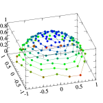
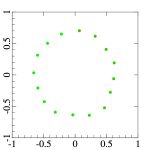
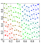
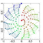
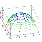
In a nutshell, it generates points on a unit 2D square first. It does it by subdividing the square into cells, and putting one point at a regular location within each cell. To randomise the samples without clumping, it reorders the columns and the rows randomly. To enhance randomness of samples, it adds some jitter to each sample, so they will be randomised even further within a substrata of the cell, which prevents it from produce banding, even if low number of cells are used. It projects the 2D sample point set to a unit radius disk using polar mapping which preserves the spatial distribution of the samples after the projection well. Next, it projects the points on the disk onto a hemisphere above the disk which ensures cosine weighted distribution.


While the overall quality of the generated points is good, the algorithm has some drawbacks, from our point of view:

To address the first problem, I replaced the scan-line ordering of samples with the good old Z-ordering (Morton code) [3]. It made possible to achieve better spatial coherence of consecutive sample points:


Obviously, it will not work on arbitrary number of rows or columns, I have chosen that because it was the simplest to experiment with. If a mapping for an arbitrary number of rows and columns is necessary, K-means clustering [4] of the hemisphere-projected center points could be useful, where 
The second problem is that the original algorithm uses some custom made hash mixing functions to generate random jitter, and permutation of rows and columns.
In their implementations, they followed the method described in Bret Mulvey’s article about Hash Functions [2] to build their permutation functions, and used hill-climbing algorithm to fine-tune their functions. Additionally, their permutation function uses a technique called “Cycle Walking” in order to reduce the output value range width of the hash function without messing up the uniformity of values (more details in [6]). The problem is that it contains a non-deterministic loop in which the number of iterations depend on the range and the produced random value.
Before we continue, some explanation might be useful here. A mixing function is a function which maps an integer input range ![[0..2^n-1]](https://s0.wp.com/latex.php?latex=%5B0..2%5En-1%5D&bg=ffffff&fg=4e4e4e&s=0&c=20201002)
Mixing functions consist of so called mixing steps performed one after another. They are reversible: their mapping is collision-free, any number of these steps can be combined together without losing overall reversibility.
i.    hash ^= constant;
ii.   hash *= constant; // if constant is odd
iii.  hash += constant;
iv.   hash -= constant;
v.    hash ^= hash >> constant;
vi.   hash ^= hash << constant;
vii.  hash += hash << constant;
viii. hash -= hash << constant;
iix.  hash = (hash  5); // if 32 bits
The proof of reversibility is discussed in more detail in the post.
(The steps can be performed on any word width, assuming that they are done in modulo 
They measured the quality of a mixing function by evaluating the so-called avalanche property. From the original post: “A function is said to satisfy the strict avalanche criterion if, whenever a single input bit is complemented (toggled between 0 and 1), each of the output bits should change with a probability of one half for an arbitrary selection of the remaining input bits.”
To quantify this property, the method calculates avalanche matrix 


To evaluate the overall fitness of a mixing function, a 
The resulting number directly reflects the quality of the function (the lower the better). This makes possible to compare two different mixing functions and decide which provides better random mapping.
This all works for arbitrary word length ![[0..m-1], m < 2^n, m \in \bf{N^+}](https://s0.wp.com/latex.php?latex=%5B0..m-1%5D%2C+m+%3C+2%5En%2C+m+%5Cin+%5Cbf%7BN%5E%2B%7D&bg=ffffff&fg=4e4e4e&s=0&c=20201002)

![[0..m-1]](https://s0.wp.com/latex.php?latex=%5B0..m-1%5D&bg=ffffff&fg=4e4e4e&s=0&c=20201002)
Since my experiments were not sensitive the exact range (I could easily go on with power of two number of sample directions), I simply omitted the requirement of having arbitrary ranges for my PRNG for a while. Later I modified the algorithm to make it possible to generate values on an arbitrary range (see below).
[1] used manually crafted mixing functions, which were fine-tuned using a small framework which employs hill-climbing to find more effective coefficients in the functions. To bring this thought one step further, I thought it might worth a try to synthesise the entire mixing function from scratch in an automated process.
To help finding a suitable function, I have implemented a small framework in C# which utilises a genetic-like algorithm in order to “evolve” good mixing functions from an initial set of randomly generated functions. The implementation relies on .NET System.Linq.Expressions [7] facility which makes possible to construct and evaluate expressions using ASTs [9] in run-time with an acceptable speed.
The outline of the algorithm is the following:
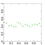
This algorithm assumes that mixing functions have a correlation between their structure and their quality, we can find a better quality mixing function by tweaking or slightly modifying an existing one. That is, we can reach better quality functions by performing simple improvements on the ones we already know. It is like our search space have some gradient-like property. If we found a mixing function which has higher quality, we can expect that it might lead to an even better one. While it is based on sole intuition (I could not find a theoretical backing to prove that assumption yet), but it apparently works fine. The chi-square test guarantees the quality of the functions we can find with this method.
Steps 3.3 and 3.4. try to help the algorithm to avoid getting stuck in a local optimum. To make it work even better, it might be useful to add an entirely new function from scratch from time to time.
The implementation is able to handle mixing functions with arbitrary power-of-two ranges, up to 32 bits, simply by applying the 
In order to make avalanche evaluation quicker, the framework uses preliminary testing of a mutated function, calculating an approximate
The algorithm led me to some interesting findings. First of all, it finds good candidates relatively quickly, even if the maximum number of allowed steps is low, like 5 or 6.
Second, it seems like that functions with good quality tend to have similar structures, a lot of those consists of alternating set of steps ii. and v., for example:
(result *= 2078995439);
(result ^= (result >> 16));
(result *= 3646025353);
(result ^= (result >> 10));
(result *= 3911234291);
(result ^= (result >> 16));
Additionally, the constants in step ii. are the best if they are large primes (or they can be factored into two primes), closer to the upper limit of the current range 
When the word width is reduced, an extra bitwise AND operation is added. For example, a 7 bit mixing function looks like this:
(result ^= (result >> 4));
(result = ((result * 67) & 127));
(result ^= (result >> 3));
(result = ((result * 101) & 127));
(result ^= (result >> 4))
The constants used in the steps are generated in respect to the word length as well, for example, the shift operators will not shift more or equal to the word length, similarly, the primes chosen for multiplications will be below the upper limit of the current range, etc.
The function will map different input values to different output values within its range, without using external data. The input value can be anything which is unique for a given invocation, like a pixel ID or similar. This makes possible to invoke the function in a parallel way, and each invocation will result in different random numbers. Moreover, it will fulfil the requirement of seeding.
The framework dumps the pool to a text file from time to time to make it possible to monitor the process, or extract the best functions in a simple way.
Here are a few functions found by the framework with their corresponding approximate 
// X^2 = 0.0042641116:
var result = seed;
(result ^= (result >> 16));
(result *= 322022693);
(result ^= (result >> 14));
(result *= 2235360983);
(result ^= (result >> 19));

// X^2 = 0.00438070260000001:
var result = seed;
(result ^= (result >> 16));
(result *= 3968764237);
(result ^= (result >> 13));
(result *= 324413651);
(result ^= (result >> 18));

// X^2 = 0.0043953292:
var result = seed;
(result ^= (result >> 16));
(result *= 2019204679);
(result ^= (result >> 12));
(result *= 559761739);
(result ^= (result >> 18));
A few other functions, which the same length limit, but 
// X^2 = 0.10595703125:
result = seed;
(result ^= (result >> 1));
(result = ((result * 15) & 255));
(result ^= (result >> 3));
(result = ((result * 221) & 255));
(result ^= (result >> 4));

// X^2 = 0.11474609375:
var result = seed;
(result ^= (result >> 1));
(result = ((result * 15) & 255));
(result ^= (result >> 3));
(result = ((result * 93) & 255));
(result ^= (result >> 4));

// X^2 = 0.12060546875:
var result = seed;
(result ^= (result >> 1));
(result = ((result * 15) & 255));
(result ^= (result >> 3));
(result = ((result * 157) & 255));
(result ^= (result >> 4));
With this framework, it is relatively easy to find different mixing functions which consist of the same kind of consecutive steps, so it is possible to pick four, and combine them and implement them vectorized on the GPU. One of those I have chosen for my experiments is implemented in the following GLSL function:
uvec4 Permute4(uint x, uint y, uint seed)
{
        uvec4 value = uvec4(x, seed, seed, seed) & uvec4(127, 127, 0xffffffff, 0xffffffff);
	value ^= value >> uvec4(3, 3, 16, 16);
	value = (value * uvec4(107, 67, 322022693, 322022693)) & uvec4(127, 127, 0xffffffff, 0xffffffff);
	value ^= value >> uvec4(3, 4, 14, 13);
	value = (value * uvec4(69, 21, 3968764237, 2235360983)) & uvec4(127, 127, 0xffffffff, 0xffffffff);
	value ^= value >> uvec4(4, 3, 19, 18);
	return value;
}
The function above is four mixing functions combined into one. They all consists of the the same kind of steps performed through all the x, y, z, w channels: x and y are 5 bit, z and w are 32 bit mixing functions. The only difference between the individual channels is the coefficients and bit masks used.
There is a problem though. Using 7 bit mixing function here will result in a repeating random pattern in sampling (which we wanted to avoid). To fix this, we can use an extra step to hide this repetition:
uvec4 Permute4(uint x, uint y, uint seed)
{
    uvec4 value = uvec4(x ^ seed, y ^ seed, seed, seed) & uvec4(127, 127, 0xffffffff, 0xffffffff);
    value ^= value >> uvec4(3, 3, 16, 16);
    value = (value * uvec4(107, 67, 322022693, 322022693)) & uvec4(127, 127, 0xffffffff, 0xffffffff);
    value ^= value >> uvec4(3, 4, 14, 13);
    value = (value * uvec4(69, 21, 3968764237, 2235360983)) & uvec4(127, 127, 0xffffffff, 0xffffffff);
    value ^= value >> uvec4(4, 3, 19, 18);
    return value;
}
The first step is “seeding” the x and y values with the values in z and w, which are unique for every unique seed value, so it does an extra, unique permutation for both x and y values.
This single function provides both row/column index permutation and jitter random values. The 5 bit functions are used for row/column permutation (for 1024 samples per texel), the 32 bit functions are for the jitter. Compared to the original ones, it is much more compact, does not use any branching, contains no loops at all, and the overall length is less than the half of the original ones. The obvious drawback is that we need a different permutation function for each word length, and functions with limited word width have short repeating period.
While it was easy to work with power of two ranges in my experiments, it was necessary to have a function which works on an arbitrary range in practice, so a single function can be used for all purposes.
Since [2] has proven that a simple modulo operation will ruin uniform distribution, I had to come up something else. I do not know whether it is a well known idea, and maybe I reinvented the wheel here, but here is my solution for this problem, which works on arbitrary ranges of ![[0..r]](https://s0.wp.com/latex.php?latex=%5B0..r%5D&bg=ffffff&fg=4e4e4e&s=0&c=20201002)


The basic idea is probably not new, it uses a few basic integer operations, when
uvec4 Rand(uvec4 seed, uvec4 range)
{
    seed ^= uvec4(seed.x >> 19, seed.y >> 19, seed.z >> 13, seed.w >> 19);
    seed *= uvec4(1619700021, 3466831627, 923620057, 3466831627);
    seed ^= uvec4(seed.x >> 16, seed.y >> 12, seed.z >> 18, seed.w >> 17);
    seed *= uvec4(175973783, 2388179301, 3077236438, 2388179301);
    seed ^= uvec4(seed.x >> 15, seed.y >> 17, seed.z >> 18, seed.w >> 18);

    uint f = seed & 0x0000ffff;
    return (r * f) >> 16
}
What it does is basically takes the full 32-bit hash value and uses it as a 16.16 fixed point integer, takes the fraction part (which represents values from ![[0..1-1/2^{16}]](https://s0.wp.com/latex.php?latex=%5B0..1-1%2F2%5E%7B16%7D%5D&bg=ffffff&fg=4e4e4e&s=0&c=20201002)
![[0...r - 1]](https://s0.wp.com/latex.php?latex=%5B0...r+-+1%5D&bg=ffffff&fg=4e4e4e&s=0&c=20201002)
The good avalanche property of the mixing function guarantees that the fraction will have uniform distribution as well (the probability of a particular bit of being either 0 or 1 is very close to 0.5 – 0.5).
It also has a nice property that it will have a full repeating period of 
It works, but it is not perfect. The distribution of mapped values are still not totally uniform: since 


![[0..2]](https://s0.wp.com/latex.php?latex=%5B0..2%5D&bg=ffffff&fg=4e4e4e&s=0&c=20201002)
![[0..2^n] = [0..15]](https://s0.wp.com/latex.php?latex=%5B0..2%5En%5D+%3D+%5B0..15%5D&bg=ffffff&fg=4e4e4e&s=0&c=20201002)
![[0..3]](https://s0.wp.com/latex.php?latex=%5B0..3%5D&bg=ffffff&fg=4e4e4e&s=0&c=20201002)
To alleviate this problem, all we need to do is add some “jitter” to the mapping:
uvec4 Rand(uvec4 seed, uvec4 range)
{
    seed ^= uvec4(seed.x >> 19, seed.y >> 19, seed.z >> 13, seed.w >> 19);
    seed *= uvec4(1619700021, 3466831627, 923620057, 3466831627);
    seed ^= uvec4(seed.x >> 16, seed.y >> 12, seed.z >> 18, seed.w >> 17);
    seed *= uvec4(175973783, 2388179301, 3077236438, 2388179301);
    seed ^= uvec4(seed.x >> 15, seed.y >> 17, seed.z >> 18, seed.w >> 18);
    uint f = seed & 0x0000ffff;
    return (range * f + (seed % range)) >> 16;
}
After the multiplication we add a small value picked from ![[0..1 / r]](https://s0.wp.com/latex.php?latex=%5B0..1+%2F+r%5D&bg=ffffff&fg=4e4e4e&s=0&c=20201002)

There is a sample implementation on Shadertoy demonstrating some of the permutation functions found by the framework. It generates not just image but sound as well. The results are quite in accordance of the theoretical expectations (or at least good enough for me :P).
With these ideas above, I have managed to adapt the original CMJS method, it became possible to generate good quality sampling direction on the GPU with low shader cost, break down the overall process into multiple batches and increase the overall ray coherence. Obviously, there are many ways to go further, but this is how far I could get on my limited time.
[1] Correlated Multi-Jittered Sampling – A. Kensler
[2] Hash Functions – B. Mulvey
[4] K-Means Clustering – Wikipedia
[6] Ciphers with Arbitrary Finite Domains – J. Black, P. Rogaway
[7] System.Linq.Expression – Microsoft .NET Framework
[8] Chi-Squared Test – Wikipedia
I have this nostalgic relation with Quake/HL series, they were one of my greatest motivation towards game tech. I really admire how they built their worlds upon simple basic concepts, like plane bounded convex polyhedron, what they call “brushes”. The idea is to take a bunch of planes (in a mathematical sense), and use them as boundaries of a convex subspace, which is the intersection of the half-spaces behind them.
The equation, 


Using a plane defined by this equation, we can classify the relation of a point to the plane. Substituting a 


Now we have a simple, handy tool to classify points against planes, so we can move on to construct convex polyhedrons using it. We know, if a 
If we setup a system of
where the 

[2] gives a detailed description how brushes are defined in Quake 1 map files. .MAP files are simple text files, listing level brushes and entities in a simple structure. A brush consists of a list of face definitions. Each face definition contains three points 


Once we have the face planes ready, we should convert them to vertices and indices in order to make them suitable to render. [2] proposes a simple method, originated in the Q1 bsp tool: they take a large ![[-4096..4096]^3](https://s0.wp.com/latex.php?latex=%5B-4096..4096%5D%5E3&bg=ffffff&fg=4e4e4e&s=0&c=20201002)
We start with a list of faces defined by vertices which form a closed (and convex) loop around the face. Two consecutive vertices define an edge. To slice a face against a plane, we test all the face edges against it. If both vertices are behind the plane, we keep both. If they are in front, then we omit them. If one of them is behind and the other is in front, we keep the one behind, and store the intersection point between the edge and the plane, instead of the vertex in front of the plane. (This method also provides an easy method to detect redundant planes, i. e. which does not influence the final brush geometry at all.)
This approach seems quite simple, but making it numerically was not entirely straightforward. After all, I came up with the following:
Let 


For all: Let
is an ordered list of clipped vertices //
: Let
is an ordered list of vertices //
after the clipping is done For all
If
is behind
is on the opposite side of
the intersection point between
. Append
: If
: Insert it where it follows the previous vertices in the right winding order
This will result in a set of faces with all the vertices in the right order, which is easy to assemble into an actual mesh.
Some images of the results, without any textures or materials for now:


The lights are simple point lights, with shadow maps using Poisson disc filter. The light energy and radius values are calculated by an empirical formula, hand tweaked to give somewhat similar results to the original lighting, using the light parameters specified the map file.
The next step is to import all the materials. To be continued….
[2] Quake Map Format
This is a test level as well as the previous one. It is a relatively large map so the portal culling comes quite in handy in this case.
I have done a quick video by request. Check it out. 🙂
Theoretically, using six shadow mapped spot lights to piece up a shadow casting point light is not a big deal. Especially if the light geometry calculation for deferred lighting is correct. Well, in my engine, it was not the case. 🙂
There was a hidden calculation error that resulted in a frustum with incorrect corner points that made it bigger than desired. This error caused no problem so far because projected mask texture on spotlights and “discard” codes in fragment shader prevented the extra pixels from being seen. But once I have used spot lights with no mask to render point light, the result was erroneous. It looked so strange and mysterious that it took few hours to find the root of the problem.
Finally, the shadows on point light are working now, and I proudly present some screenshots here.


In an earlier post, I have written that I have implemented Lua script support in the engine. Now it reached its full power since I have added a proper callback mechanism to it. It makes possible for the triggers in the engine to call user specified Lua functions on firing. Unfortunately, SWIG does not help to implement such callbacks, so I had to do it by myself.

I have added a new technique called … I’d rather not write it down again…. So, the great thing is that it mimics reflections on shiny surfaces using a simple, but yet quite accurate approximation based on environment cubemap textures.
For more details, see http://www.gamedev.net/topic/568829-box-projected-cubemap-environment-mapping.
The hard part was to find a hidden bug in the engine that prevented me to render in-scene cubemap snapshots using a dedicated off-screen compositor chain. But eventually I have managed to find it and it seems that it worth the effort.
The engine automatically places light probes in each room in the level at load time, then it renders a fully lit HDR cubemap texture for each of them. The engine uses these cubemaps and some extra parameters assigned to the probes, to calculate the reflections with the aforementioned method.
First I have experimented with a similar idea that uses spheres to distort the cubemap look-up coordinates, but it was inaccurate. BPCEM gives a more accurate results in box-shaped rooms.
There are some images with the results:


A demo video:
Now the exporter supports nearly all the things required to create an indoor level for the engine. After several days of work and a helping artistic hand from Endre Barath (etyekfilm.hu), we have created the first explorable level in the engine. There is no much to say, aside from that it was a large amount of work from me to make things work. It was mostly debugging and optimization but some new features were also added like color grading, tangent/bitangent generation at loading time, and multi-material support per model.
Of course, the job is not finished yet, so many things should be fixed, but there is a short video showing the results.
Currently, I am working on an exporter for Blender that greatly speeds up content creation process for the engine. It is not complete yet, but I thought that it worth a post. It supports meshes, instances, materials, textures, point and spotlights.
The exporter saves all meshes in obj format (ugly, I know, but works). It creates Merlin3D scene files with all mesh and light instances. Moreover, it generates effects files automatically, configuring the call of an appropriate GLSL shader and configures the parameters for it. Some of these parameters are the textures taken from texture slots in Blender materials. The exporter supports diffuse, normal, specular and glow maps at this time, but support for further texture types can be easily added. There are also shader parameters coming from material texture settings like specular and glow coefficient, and things like that.
The script extracts several light parameters, such as color, energy, radius (or distance in Blender terminology) spotlight angle or falloff type.
There are a lot of things missing, but the results achieved now are promising… 🙂
Finally, let’s see some screenshots.


Again, I had some time to play with the code. And again, I have rewritten the game object representation structure to make things simpler inside the engine. I have added a new object type “function”. It is a non-rendering scene node, making different things to other objects. It can heal, give damage, etc., and teleport. It is activated a physics trigger by touching.
I have implemented some teleports in the scene using these new objects. The following video demonstrates how it works.
Experiences with realtime rendering, game engine programming, C++, and 3D APIs.
